Combinations, permutations and simulations
I’ve been sitting on this post for a number of weeks, so I hope that it still maintains a common thread throughout. The thread that I pull at, in this post, is one of understanding. I recently squinted at the binomial distribution and realized that I didn’t fundamentally understand many of the concepts that go into it. I briefly encountered it during my undergraduate degree and I could mechanically do all of the related proofs, but I didn’t “get it”. Throughout this post, I cover all of the concepts that go into understanding what makes up the probability distribution, but not in a mathematically rigorous way. I’m aiming more for pedagogy. I’ve also done my best to link out for further reading, if my explanations fall short.
Probability
Probability1 is a very broad topic, but – for this post – you will need to understand two things.
- The probability of all possible outcomes in an experiment must sum to .
- The probability of two or more independent events having a specific outcome is equal to the product of their probabilities.
The first point can be seen as axiomatic. Probabilities range from , as they represent percentages from . We don’t expect things to happen less than of the time or more than of the time.
The second point is a little bit more complicated to understand, so let’s use the common example of repeatedly flipping a coin. A fair coin is one that lands on heads of the time and tails, otherwise. This is not a coin that repeatedly lands on heads and then tails in succession, but one that has that proportion after very many coin flips.
If you were to draw out a tree representing the result of each coin flip given three successive flips you’d get the following:
Noticeably you’d see that, at the leaves, I’ve given each event a value of . We don’t have to know that we can multiply the probabilities to work this out. We know that we have eight possible routes that our experiment could take, and we know that each path is equally likely to occur, from the premise. From (1.), we also know that our probabilities must add up to . So, with eight possible outcomes, we must have a chance of for each event to occur. Algebraically, this explanation is given as:
This is, however, only an example. I haven’t covered why this is the case even for events that have a different number of outcomes. For example, imagine I flip a coin and then roll a 6-sided die. If you struggle to picture things in your head, like me, I would recommend drawing this case out. I’d also recommend following along with a pen and paper for most of this post whenever you need to convince yourself.
As an aside, Venn diagrams2 are another handy way of visualizing sets and probability for these more base concepts.
Permutations
With some introductory probability concepts in our pocket, we’ll need to build up some primitives for counting. I don’t personally find the equations we end up with intuitive, so I’ve worked on some animations as concrete examples.
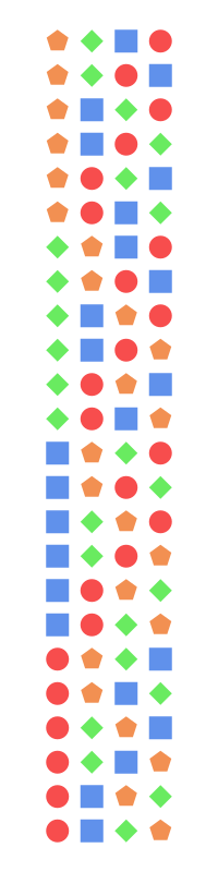
To set the scene, we need to imagine that we have a number of things and we want to figure out how many different ways we can order those things. I’ve opted for some colourful shapes. The most straightforward way to do so is start with some large-enough number of shapes and draw out all of the possibilities. Let’s pick four shapes. We get the following:
Well, that’s daunting. However, notice that the first column doesn’t change much. In fact, if we split up our result into four groups where the first column doesn’t change we end up with four groups of six rows each. For each group, give the first four elements a number from . Then, give the appropriate number to the following rows. You’ll notice that all four groups have an identical relative ordering. In other words, if we stop considering their exact identity (in this case, colourful shapes), then there is no difference in their order. So, the number of ways to sort these groups is:
Since they all have the same relative ordering, we just need to consider one of these groups for the remaining ordering. Since the first element never changes, we can strip it off. Interestingly, the same pattern emerges. We get groups with identical relative ordering. This continues all the way down to which cannot be relatively ordered to nothing, so it’s simply . The following animation demonstrates this process:
More simply, we can now picture this process as taking our set of things and putting them into the same number of slots. Another way to think of it is to, at each step, think of how many different elements fit into the current slot. Once you’ve chosen one, your set of options decreases by one.
What we have discovered is known as the factorial. The definition of the factorial is given as:
This is the most trivial version of what’s known as a permutation. Generally, a permutation is the number of ways to sort things into slots. Since I like to start with an example, observe the following case where we have items and we want to sort them into slots.
You’ll notice we sort of “stop doing the factorial” after the . In effect, we want to divide out from . So, we want some function that gives us:
This can be more precisely written as:
Combinations
We defined permutations so that we have the tools we need for the next concept: Combinations. Combinations are a way of taking some number of unique things and seeing how many different ways we can throw them into a bag. Unlike with permutations and the previously mentioned slots, we don’t care how the elements are sorted in the bag. The simplest example of that is to throw everything we have into the bag. There is only one way to throw everything we have into the bag – ignoring how they are sorted within.
Similarly to permutations, we’ll use the symbol for the number of things and for the number of things that get thrown into this bag. We actually start in a similar way as we did for the permutation case. The difference is that, once we have our items in the bag, we want to divide out the different ways we can sort them inside the bag. So, since we have items in the bag which are currently concerned with their order, we discover that we have another permutation! Technically, we have the trivial case which is just a factorial. So, putting that all together we can define the combination as:
Let’s validate that this works for the trivial case depicted above:
Binomial distribution
The binomial distribution is concerned with a situation where we have independent events with a success rate of (a probability). The binomial distribution is known as a discrete probability distribution3. That is, it’s a probability distribution that only has integer values as inputs. The function for producing the probability for each possible outcome of a discrete distribution is known as a probability mass function (PMF)4.
We can define our PMF as 5. The symbol I haven’t introduced, , is the number of successes. This is the discrete/integer value mentioned above.
Let’s first think about how many possible events there are. Should we use a combination or permutation, or something else? Well, we probably don’t want to encode the order of events into our equation. We know that the events are independent, so we really just care about how many “trials (things) there are in the success bag”. So, we have different cases where the success count is .
Great, so now we need to determine the probability of these events. We know that they are independent, so we can multiply them. In other words, we can define the probability of successes for trials as:
This is only the probability for exactly one such outcome however. We just aren’t writing them in order, since they’re independent and multiplication is commutative.
To elaborate, say we had two successes and then a failure or we had one success, a failure and then a success. These would occur with probabilities and , since they are independent events. These are equivalent. Now, note that this is not the order of the successes (which doesn’t matter), but rather just the possible branches in our experiment that have the exact same number of successes. Think back to the coin flip example described right at the beginning. We could have HHT, HTH, or THH, but ultimately we have to same number of heads and tails for these events – which you can translate as the same number of successes and failures, where .
So, putting it all together, we have our PMF as:
Combinations have a more common alternative syntax, so you’ll often see something like:
It’s often spoken as “ choose ”.
Simulations
Let’s take this a step further. After all of this, can we validate that we’ve ended up with a good formula for the binomial distribution’s PMF? The heading gives it away, but the answer is to run a simulation. At least for me, this gives the extra bit of confidence in my understanding. There are many other analytical methods for validating it, but a simulation is straightforward and usually easier to throw together.
Firstly, let’s validate the analytical solution we have. Is this a valid PMF? Well, we just need to add up the probability for every valid value of . If this is valid, then the sum of all values for our PMF should equal . We know that , by definition. So, let’s write a Python program for a handful of trials varying and .
from math import comb, pow

def binomial(s: int, n: int, p: float):
    return comb(n, s) * pow(p, s) * pow(1 - p, n - s)

for n in [1, 5, 10, 20]:
    for p in [0.2, 0.3, 0.5, 0.8]:
        pmf_sum = sum(binomial(s, n, p) for s in range(0, n+1))
        print("n={}, p={}, pmf_sum={:.2f}".format(n, p, pmf_sum))
Fortunately, all we needed was the built in math module! For me, these values output (or a value very close to it). This means we have something that passes the definition of a PMF.
Now, let’s write a program that is not at all aware of the binomial distribution or what “PMF” means. Python provides a module for producing random values6 which allows us to simulate trials that have some success rate. We can simulate many runs of our experiment in which trials have a success rate of .
from collections import defaultdict
import random
p = 0.8 # success rate
n = 10 # trials
iterations = 100000
buckets = defaultdict(lambda: 0, {})
for _ in range(iterations):
successes = sum([random.random() <= p for _ in range(n)])
buckets[successes] += 1
print("successes,proportion")
for i in range(n + 1):
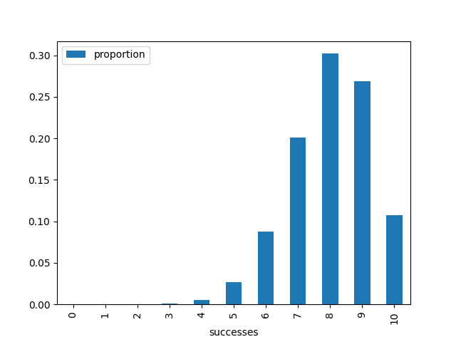
print("{},{}".format(i, buckets[i] / iterations))
I’ve graphed the output of the proportion of successes.

I like to separate the data production from graphing the output, in case I want
to tweak either side of the process. So, to generate the above graph, I run the
script to generate the data as python3 data.py > results.csv. Then, I run the
following snippet to get the graph.
import matplotlib.pyplot as plt
import pandas as pd

data = pd.read_csv("./results.csv")
data.plot(x = 'successes')
plt.show()
Now, let’s compare that to the analytical solution for the PMF of the binomial distribution:
import matplotlib.pyplot as plt
import numpy as np
from math import comb, pow

def binomial(s: int, n: int, p: float):
    return comb(n, s) * pow(p, s) * pow(1 - p, n - s)

n = 10
p = 0.8

x = np.linspace(0, n, n + 1)
y = np.array([binomial(int(xi), n, p) for xi in x])

print("successes,proportion")
for i in range(n + 1):
    print("{:g},{:.5g}".format(x[i], y[i]))
Graphing this data, we get the following:
Notice how these graphs are near identical. I’ve tabulated the values below just to show you that they are, in fact, different.
| Successes | Simulation | Theory |
|---|---|---|
| 0 | 0.0 | 1.024e-07 |
| 1 | 1e-05 | 4.096e-06 |
| 2 | 6e-05 | 7.3728e-05 |
| 3 | 0.00091 | 0.00078643 |
| 4 | 0.00588 | 0.005505 |
| 5 | 0.02579 | 0.026424 |
| 6 | 0.08752 | 0.08808 |
| 7 | 0.20031 | 0.20133 |
| 8 | 0.304 | 0.30199 |
| 9 | 0.26848 | 0.26844 |
| 10 | 0.10704 | 0.10737 |
This is not a rigorous proof, but it demonstrates some of the power of simulations as a tool for understanding. If you lower the number of iterations for the simulation, it becomes more inaccurate. But, as the iterations are increased, it tends more towards the graph of the PMF. I’ll end this post with a short animation of a simulation with increasing iterations over time compared to the PMF:
Footnotes
-
https://en.wikipedia.org/wiki/Probability_distribution#Discrete_probability_distribution ↩
-
There are a number of ways to define this function, but I’m sticking to a more general mathematical notation. You may notice I’ve done the same for most of this post. ↩
-
These pseudo-random values need to be uniformly distributed, but discussion of that is beyond the scope of this post. ↩